Tidy Tuesday 08/10/2019 International Powerlifiting

Data description

From From TidyTuesdays github:

This week’s data is from Open Powerlifting.
Wikipedia has many details around the sport itself, as well as more details around the 3 lifts (squat, bench, and deadlift).
Credit to Nichole Monhait for sharing this fantastic open dataset. Please note this is a small subset of the data limited to IPF (International Powerlifting Federation) events, the full dataset with many more columns and alternative events can be found as a .csv at https://openpowerlifting.org/data. The full dataset has many more federations, ages, and meet types but is >250 MB.
A nice analysis of this dataset for age-effects in R can be found at Elias Oziolor’s Blog

Import data and packages

library(tidyverse)
library(lubridate)
library(Cairo)

ipf_data <- readr::read_csv("https://raw.githubusercontent.com/rfordatascience/tidytuesday/master/data/2019/2019-10-08/ipf_lifts.csv")

size_df <- df_clean %>% 
  select(name:weight_class_kg, starts_with("best"), place, date, federation, meet_name)  %>% 
  filter(!is.na(date)) %>% 
  filter(federation == "IPF") %>% 
  object.size()

ipf_data <- df_clean %>% 
  select(name:weight_class_kg, starts_with("best"), place, date, federation, meet_name)  %>% 
  filter(!is.na(date)) %>% 
  filter(federation == "IPF")

print(size_df, units = "MB")

## 6.2 Mb

ipf_data %>% 
  write_csv("ipf_lifts.csv")

Data

str(ipf_data)

## Classes 'spec_tbl_df', 'tbl_df', 'tbl' and 'data.frame': 41152 obs. of  16 variables:
##  $ name            : chr  "Hiroyuki Isagawa" "David Mannering" "Eddy Pengelly" "Nanda Talambanua" ...
##  $ sex             : chr  "M" "M" "M" "M" ...
##  $ event           : chr  "SBD" "SBD" "SBD" "SBD" ...
##  $ equipment       : chr  "Single-ply" "Single-ply" "Single-ply" "Single-ply" ...
##  $ age             : num  NA 24 35.5 19.5 NA NA 32.5 31.5 NA NA ...
##  $ age_class       : chr  NA "24-34" "35-39" "20-23" ...
##  $ division        : chr  NA NA NA NA ...
##  $ bodyweight_kg   : num  67.5 67.5 67.5 67.5 67.5 67.5 67.5 90 90 90 ...
##  $ weight_class_kg : chr  "67.5" "67.5" "67.5" "67.5" ...
##  $ best3squat_kg   : num  205 225 245 195 240 ...
##  $ best3bench_kg   : num  140 132 158 110 140 ...
##  $ best3deadlift_kg: num  225 235 270 240 215 230 235 335 310 295 ...
##  $ place           : chr  "1" "2" "3" "4" ...
##  $ date            : Date, format: "1985-08-03" "1985-08-03" ...
##  $ federation      : chr  "IPF" "IPF" "IPF" "IPF" ...
##  $ meet_name       : chr  "World Games" "World Games" "World Games" "World Games" ...
##  - attr(*, "spec")=
##   .. cols(
##   ..   name = col_character(),
##   ..   sex = col_character(),
##   ..   event = col_character(),
##   ..   equipment = col_character(),
##   ..   age = col_double(),
##   ..   age_class = col_character(),
##   ..   division = col_character(),
##   ..   bodyweight_kg = col_double(),
##   ..   weight_class_kg = col_character(),
##   ..   best3squat_kg = col_double(),
##   ..   best3bench_kg = col_double(),
##   ..   best3deadlift_kg = col_double(),
##   ..   place = col_character(),
##   ..   date = col_date(format = ""),
##   ..   federation = col_character(),
##   ..   meet_name = col_character()
##   .. )

I want to find if any equipment is preferred by a certain gender or age group.

facet_titles <- c(
  'best3squat_kg' = 'Squat',
  'best3bench_kg' = 'Bench',
  'best3deadlift_kg' = 'Deadlift'
)


ipf_data %>% 
  select(sex, age, best3squat_kg, best3bench_kg, best3deadlift_kg) %>% 
  pivot_longer(-c(sex, age), names_to = 'type', values_to = 'best') %>% 
  filter(best > 0) %>% 
  mutate(sex = factor(sex, levels = c('M','F'), ordered = TRUE)) %>% 
  ggplot(aes(age, best)) +
  geom_point(alpha = 1/20, color = 'darkslategrey') +
  geom_smooth(aes(color = sex), se = FALSE) +
  facet_wrap(~type,
             labeller = as_labeller(facet_titles)) +
  scale_color_manual(values = c('blue2', 'red1'),
                     name = 'Gender') +
  xlab('Age') +
  ylab('Weight(kg)') +
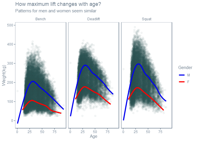
  labs(title = 'How maximum lift changes with age?',
      subtitle = 'Patterns for men and women seem similar') + 
  theme_bw() + 
  theme(panel.grid.major = element_blank(),
        panel.grid.minor = element_blank(),
        strip.background = element_blank(),
        strip.placement = 'outside',
        panel.border = element_rect(color = 'lightslategrey'),
        title = element_text(colour = "slategrey"),
        legend.text = element_text(colour = "slategrey"),
        strip.text = element_text(color = 'slategrey'),
        axis.ticks = element_line(color = 'lightslategrey'),
        axis.text = element_text(color = 'lightslategrey')
        )