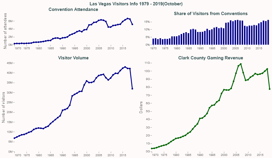
Makeover Monday 04/11/2019 Las Vegas Convention Attendance & Visitor Traffic
2019/W45: Las Vegas Convention Attendance & Visitor Traffic
Data from here
Interactive plot
Load packages and import data
import pandas as pd
import altair as alt
df = pd.read_csv('https://query.data.world/s/n3pj6omagl3flwxbzs6mblkjroi45y', sep='\t',
                 thousands=',', encoding='utf_16_le')
df.head()
| Year | Months | Visitor Volume | Convention Attendance | Room Inventory | Midweek Occupancy Percentage | Weekend Occupancy Percentage | Overall Occupancy Percentage | LVCVA Room Tax Collections | En/Deplaned Air Passenger | Clark County Gaming Revenue | |
|---|---|---|---|---|---|---|---|---|---|---|---|
| 0 | 1970 | 12 | 6787650 | 269129 | 25430 | NaN | NaN | 68.00% | 3751265.0 | 4086973 | 369,286,977 |
| 1 | 1971 | 12 | 7361783 | 312347 | 26044 | NaN | NaN | 78.30% | 4241630.0 | 4102285 | 399,410,972 |
| 2 | 1972 | 12 | 7954748 | 290794 | 26619 | NaN | NaN | 81.20% | 4770716.0 | 4608764 | 476,126,720 |
| 3 | 1973 | 12 | 8474727 | 357248 | 29198 | NaN | NaN | 84.40% | 5556312.0 | 5397017 | 588,221,779 |
| 4 | 1974 | 12 | 8664751 | 311908 | 32826 | NaN | NaN | 78.70% | 6559315.0 | 5944433 | 684,714,502 |
So, every year has 12 months?
df.query('Months != 12')
| Year | Months | Visitor Volume | Convention Attendance | Room Inventory | Midweek Occupancy Percentage | Weekend Occupancy Percentage | Overall Occupancy Percentage | LVCVA Room Tax Collections | En/Deplaned Air Passenger | Clark County Gaming Revenue | |
|---|---|---|---|---|---|---|---|---|---|---|---|
| 49 | 2019 | 10 | 31880200 | 5164500 | 149050 | 86.7% | 95.1% | 89.2% | NaN | 38500861 | $7,753,090,000 |
Yes, except for the current one, 2019.
And a quick describe.
df.describe(include='all')
| Year | Months | Visitor Volume | Convention Attendance | Room Inventory | Midweek Occupancy Percentage | Weekend Occupancy Percentage | Overall Occupancy Percentage | LVCVA Room Tax Collections | En/Deplaned Air Passenger | Clark County Gaming Revenue | |
|---|---|---|---|---|---|---|---|---|---|---|---|
| count | 50.00000 | 50.000000 | 5.000000e+01 | 5.000000e+01 | 50.000000 | 37 | 37 | 50 | 4.900000e+01 | 5.000000e+01 | 50 |
| unique | NaN | NaN | NaN | NaN | NaN | 27 | 27 | 44 | NaN | NaN | 50 |
| top | NaN | NaN | NaN | NaN | NaN | 81.60% | 93.50% | 89.10% | NaN | NaN | 476,126,720 |
| freq | NaN | NaN | NaN | NaN | NaN | 4 | 4 | 2 | NaN | NaN | 1 |
| mean | 1994.50000 | 11.960000 | 2.539469e+07 | 3.051318e+06 | 92756.660000 | NaN | NaN | NaN | 9.983591e+07 | 2.589947e+07 | NaN |
| std | 14.57738 | 0.282843 | 1.256754e+07 | 2.224790e+06 | 45366.843933 | NaN | NaN | NaN | 8.887047e+07 | 1.544387e+07 | NaN |
| min | 1970.00000 | 10.000000 | 6.787650e+06 | 2.691290e+05 | 25430.000000 | NaN | NaN | NaN | 3.751265e+06 | 4.086973e+06 | NaN |
| 25% | 1982.25000 | 12.000000 | 1.204321e+07 | 8.432370e+05 | 50834.750000 | NaN | NaN | NaN | 1.907066e+07 | 1.030479e+07 | NaN |
| 50% | 1994.50000 | 12.000000 | 2.860824e+07 | 2.804525e+06 | 89303.000000 | NaN | NaN | NaN | 7.687679e+07 | 2.743886e+07 | NaN |
| 75% | 2006.75000 | 12.000000 | 3.737544e+07 | 5.106924e+06 | 133126.250000 | NaN | NaN | NaN | 1.648218e+08 | 4.119840e+07 | NaN |
| max | 2019.00000 | 12.000000 | 4.293610e+07 | 6.646200e+06 | 150593.000000 | NaN | NaN | NaN | 2.825960e+08 | 4.971658e+07 | NaN |
Some numeric values are not in the right type. So I’ll take a look and transform them.
df['Clark County Gaming Revenue']
0        369,286,977
1        399,410,972
2        476,126,720
3        588,221,779
4        684,714,502
5        770,336,695
6        845,975,652
7      1,015,463,342
8      1,236,235,456
9      1,423,620,102
10     1,617,194,799
11     1,676,148,606
12     1,751,421,394
13     1,887,451,717
14     2,008,155,460
15     2,256,762,736
16     2,431,237,168
17     2,789,336,000
18     3,136,901,000
19     3,430,851,000
20     4,104,001,000
21     4,152,407,000
22     4,381,710,000
23     4,727,424,000
24     5,430,651,000
25     5,717,567,000
26     5,783,735,000
27     6,152,415,000
28     6,346,958,000
29     7,210,700,000
30     7,671,252,000
31     7,636,547,000
32     7,630,562,000
33     7,830,856,000
34     8,711,426,000
35     9,717,322,000
36    10,630,387,000
37    10,868,464,000
38     9,796,749,000
39     8,838,261,000
40     8,908,574,000
41     9,222,677,000
42     9,399,845,000
43     9,674,404,000
44     9,553,864,000
45     9,617,671,000
46     9,713,930,000
47     9,978,503,000
48    10,249,964,000
49    $7,753,090,000
Name: Clark County Gaming Revenue, dtype: object
One value has a $ that is impeding the transformation to numeric. I’ll fix this and alo some other changes to make the data looks better in the plot and creating a new column to see proportion as
df_clean = df.copy()
df_clean['Clark County Gaming Revenue'] = pd.to_numeric(df_clean['Clark County Gaming Revenue'].str.replace('[,$]',''),
                                                       downcast='integer')
df_clean['Midweek Occupancy Percentage'] = pd.to_numeric(df_clean['Midweek Occupancy Percentage'].str.replace('%',''))
df_clean['Weekend Occupancy Percentage'] = pd.to_numeric(df_clean['Weekend Occupancy Percentage'].str.replace('%',''))
df_clean['Overall Occupancy Percentage'] = pd.to_numeric(df_clean['Overall Occupancy Percentage'].str.replace('%',''))

#Create new column
df_clean['Proportion'] = df_clean['Convention Attendance']/df_clean['Visitor Volume']
df_clean['Year'] = pd.to_datetime(df_clean['Year'], format='%Y')

df_clean.dtypes
Year                            datetime64[ns]
Months                                   int64
Visitor Volume                           int64
Convention Attendance                    int64
Room Inventory                           int64
Midweek Occupancy Percentage           float64
Weekend Occupancy Percentage           float64
Overall Occupancy Percentage           float64
LVCVA Room Tax Collections             float64
En/Deplaned Air Passenger                int64
Clark County Gaming Revenue              int64
Proportion                             float64
dtype: object
So the values are now in the correct format. Let’s see if there are NAs and make the visualization.
df_clean.isnull().sum()
Year                             0
Months                           0
Visitor Volume                   0
Convention Attendance            0
Room Inventory                   0
Midweek Occupancy Percentage    13
Weekend Occupancy Percentage    13
Overall Occupancy Percentage     0
LVCVA Room Tax Collections       1
En/Deplaned Air Passenger        0
Clark County Gaming Revenue      0
Proportion                       0
dtype: int64
Three variables have NA values but I’ll redo the original plot with two plots.
brush = alt.selection_interval(encodings=['x'],empty='all')

base_line_bar = alt.Chart(df_clean).encode(
    x=alt.X('Year', title=None),
    color=alt.condition(brush, alt.ColorValue('darkblue'), alt.ColorValue('gray')),
    tooltip=alt.Tooltip('year(Year):N')
).add_selection(
    brush
)

#Convention line/scatter
chart_convention = base_line_bar.mark_line(point=True, size=3).encode(
    y=alt.Y('Convention Attendance', title='Number of attendees',
           axis=alt.Axis(format='~s'))
).properties(
    title='Convention Attendance',
    width=400,
    height=300*14/45
)

#Visitor line/scatter
chart_visitors = base_line_bar.mark_line(point=True, size=3).encode(
    y=alt.Y('Visitor Volume', title='Number of visitors',
           axis=alt.Axis(format='~s'))
).properties(
    title='Visitor Volume',
    width=400,
    height=300
)

#Conventionas proportion of total visitors
chart_proportion = base_line_bar.mark_bar().encode(
    y=alt.Y('Proportion', title=None,
           axis=alt.Axis(format='%'))
).properties(
    title='Share of Visitors from Conventions',
    width=400,
    height=300*14/45
)

#Gaming Spending
chart_spending = base_line_bar.mark_line(
    point=True, size=3
).encode(
    y=alt.Y('Clark County Gaming Revenue', title='Dollars',
           axis=alt.Axis(format='~s')),
    color=alt.condition(brush, alt.ColorValue('darkgreen'), alt.ColorValue('gray'))
).properties(
    title='Clark County Gaming Revenue',
    width=400,
    height=300
)

final_chart = (
    (
        chart_convention & chart_visitors
    ) | (
        chart_proportion & chart_spending
    )
).properties(
    title = 'Las Vegas Visitors Info 1979 - 2019(October)'
).configure(
    background='Snow'
).configure_axis(
    grid=False,
    domain=False,
    titleFontSize=13,
    titleFontWeight='normal',
    titleColor='dimgray',
    labelColor='dimgray'
).configure_view(
    strokeWidth=0
).configure_title(
    fontSize=15,
    anchor='middle',
    color='darkslategray'
)

final_chart.save("../docs/assets/images/2019_11_04_MM.png")
final_chart.save('2019_11_04_MM.html')
final_chart