Tidy Tuesday 29/10/2019 NYC Squirrel Census
Data description
From From TidyTuesdays github:
This week’s data is from the NYC Squirrel Census - raw data at NY Data portal.
H/t to Sara Stoudt for sharing this data, and Mine Cetinkaya-Rundel for her squirrel data package using the same data.
CityLab’s Linda Poon wrote an article using this data.
Data importing
library(tidyverse)
Now reading the data (using RCurl because my connection with regular curl is weird)
nyc_squirrels <- readr::read_csv(RCurl::getURL("https://raw.githubusercontent.com/rfordatascience/tidytuesday/master/data/2019/2019-10-29/nyc_squirrels.csv"))
Quick look
glimpse(nyc_squirrels)
## Observations: 3,023
## Variables: 36
## $ long                                       <dbl> -73.95613, -73.95704,…
## $ lat                                        <dbl> 40.79408, 40.79485, 4…
## $ unique_squirrel_id                         <chr> "37F-PM-1014-03", "37…
## $ hectare                                    <chr> "37F", "37E", "02E", …
## $ shift                                      <chr> "PM", "PM", "AM", "PM…
## $ date                                       <dbl> 10142018, 10062018, 1…
## $ hectare_squirrel_number                    <dbl> 3, 3, 3, 5, 1, 2, 2, …
## $ age                                        <chr> NA, "Adult", "Adult",…
## $ primary_fur_color                          <chr> NA, "Gray", "Cinnamon…
## $ highlight_fur_color                        <chr> NA, "Cinnamon", NA, N…
## $ combination_of_primary_and_highlight_color <chr> "+", "Gray+Cinnamon",…
## $ color_notes                                <chr> NA, NA, NA, NA, NA, N…
## $ location                                   <chr> NA, "Ground Plane", "…
## $ above_ground_sighter_measurement           <chr> NA, "FALSE", "4", "3"…
## $ specific_location                          <chr> NA, NA, NA, NA, NA, N…
## $ running                                    <lgl> FALSE, TRUE, FALSE, F…
## $ chasing                                    <lgl> FALSE, FALSE, FALSE, …
## $ climbing                                   <lgl> FALSE, FALSE, TRUE, T…
## $ eating                                     <lgl> FALSE, FALSE, FALSE, …
## $ foraging                                   <lgl> FALSE, FALSE, FALSE, …
## $ other_activities                           <chr> NA, NA, NA, NA, "unkn…
## $ kuks                                       <lgl> FALSE, FALSE, FALSE, …
## $ quaas                                      <lgl> FALSE, FALSE, FALSE, …
## $ moans                                      <lgl> FALSE, FALSE, FALSE, …
## $ tail_flags                                 <lgl> FALSE, FALSE, FALSE, …
## $ tail_twitches                              <lgl> FALSE, FALSE, FALSE, …
## $ approaches                                 <lgl> FALSE, FALSE, FALSE, …
## $ indifferent                                <lgl> FALSE, FALSE, TRUE, F…
## $ runs_from                                  <lgl> FALSE, TRUE, FALSE, T…
## $ other_interactions                         <chr> NA, "me", NA, NA, NA,…
## $ lat_long                                   <chr> "POINT (-73.956134493…
## $ zip_codes                                  <dbl> NA, NA, NA, NA, NA, N…
## $ community_districts                        <dbl> 19, 19, 19, 19, 19, 1…
## $ borough_boundaries                         <dbl> 4, 4, 4, 4, 4, 4, 4, …
## $ city_council_districts                     <dbl> 19, 19, 19, 19, 19, 1…
## $ police_precincts                           <dbl> 13, 13, 13, 13, 13, 1…
I’ll look at how high the squirrels go.
How high care the squirrels?
nyc_squirrels %>%
  select(location, above_ground_sighter_measurement) %>%
  summary()
##    location         above_ground_sighter_measurement
##  Length:3023        Length:3023
##  Class :character   Class :character
##  Mode  :character   Mode  :character
Not a lot of sense in above_ground being a character, let’s change that. And since I’ll be making two bar plots it’s easier to make two datasets.
squirrels_above_below <- nyc_squirrels %>%
  select(location) %>%
  filter(!is.na(location)) %>%
  count(location, name = "location_prop") %>%
  mutate(location_prop = location_prop/sum(location_prop))

squirrels_above_below
## # A tibble: 2 x 2
##   location     location_prop
##   <chr>                <dbl>
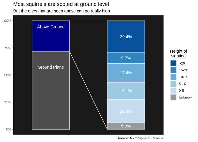
## 1 Above Ground         0.285
## 2 Ground Plane         0.715
Now making a data frame for the squirrels sighter measurements.
squirrels_sight_measures <- nyc_squirrels %>%
  filter(location == "Above Ground") %>%
  select(above_ground_sighter_measurement) %>%
  mutate(above_ground_sighter_measurement = parse_number(above_ground_sighter_measurement))

squirrels_sight_measures %>% summary()
##  above_ground_sighter_measurement
##  Min.   :  0.00
##  1st Qu.:  5.00
##  Median : 10.00
##  Mean   : 15.21
##  3rd Qu.: 20.00
##  Max.   :180.00
##  NA's   :50
So the values have 50 NAs, and mostly distributed around 5 and 20.
squirrels_sight_measures <- squirrels_sight_measures %>%
  mutate(height_category = case_when(
    is.na(above_ground_sighter_measurement) ~ "Unknown",
    above_ground_sighter_measurement < 5 ~ "0-5",
    above_ground_sighter_measurement < 10 ~ "5-10",
    above_ground_sighter_measurement < 15 ~ "10-15",
    above_ground_sighter_measurement < 20 ~ "15-20",
    above_ground_sighter_measurement >= 20 ~ ">20"
  ),
  height_category = factor(height_category, levels = c("Unknown", "0-5", "5-10",
                                                  "10-15", "15-20", ">20"),
                           ordered = TRUE)
  ) %>%
  count(height_category, name = "above_prop") %>%
  mutate(above_prop = above_prop/sum(above_prop))
Great, so now I’ll make a stacked bar chart.
ggplot() +
  geom_col(data = squirrels_above_below,
           aes(x = 1, y = location_prop, fill = location),
           position ="fill", width = .5, color = "white") +
  geom_text(data = squirrels_above_below,
            aes(x = 1, y = location_prop,  label = location, group = location),
            color = "white", position = position_stack(.8, reverse = FALSE)) +
  geom_col(data = squirrels_sight_measures,
           aes(x = 2, y = above_prop, fill = height_category),
           position = position_fill(reverse = TRUE), width = .5, color = "white") +
  geom_text(data = squirrels_sight_measures,
           aes(x = 2, y = above_prop, label = scales::percent(above_prop)),
           color = "white", position = position_stack(.5)) +
  geom_segment(data = squirrels_above_below %>% filter(location == "Ground Plane"),
               aes(x = 1 + .5/2, xend = 2-.5/2, y = location_prop, yend = 0),
               color = "white") +
  geom_segment(aes(x = 1 + .5/2, xend = 2-.5/2, y = .999, yend = .999),
               color = "white") +
  labs(
    title = "Most squirrels are spoted at ground level",
    subtitle = "But the ones that are seen above can go really high",
    caption = "Source: NYC Squirrel Census"
  ) +
  scale_fill_manual("Height of\n sighting",
                    values = c(">20" = "#08519c", "15-20" = "#3182bd",
                               "10-15" = "#6baed6", "5-10" = "#9ecae1",
                               "0-5" = "#c6dbef", "Unknown" = "grey60",
                               "Above Ground" = "darkblue",
                               "Ground Plane" = "grey30"),
                    breaks=c(">20", "15-20", "10-15", "5-10", "0-5",
                             "Unknown", NULL, NULL)) +
  scale_y_continuous(NULL, labels = scales::percent) +
  scale_x_continuous(NULL, labels = NULL, breaks = NULL, expand = c(.1,.1)) +
    theme(panel.background = element_rect(fill = "grey10"),
          panel.grid = element_blank())