Tidy Tuesday 03/12/2019 Philadelphia Parking Violations

Data description

From From TidyTuesdays github:

This week’s data is from Open Data Philly - there is over 1 GB of data, but I have filtered it down to <100 MB due to GitHub restrictions. I accomplished this mainly by filtering to data for only 2017 in Pennsylvania that had lat/long data. If you would like to use the entire dataset, please see the link above.

H/t to Jess Streeter for sharing this week’s data!

Some visualizations from Philly Open Data and a news article by NBC Philadelphia.

Packages and data reading

library(tidyverse)
library(patchwork)

tickets <- readr::read_csv("https://raw.githubusercontent.com/rfordatascience/tidytuesday/master/data/2019/2019-12-03/tickets.csv")

Quick look

tickets %>% glimpse()

## Observations: 1,260,891
## Variables: 7
## $ violation_desc <chr> "BUS ONLY ZONE", "STOPPING PROHIBITED", "OVER TIME L...
## $ issue_datetime <dttm> 2017-12-06 12:29:00, 2017-10-16 18:03:00, 2017-11-0...
## $ fine           <dbl> 51, 51, 26, 26, 76, 51, 36, 36, 76, 26, 26, 301, 36,...
## $ issuing_agency <chr> "PPA", "PPA", "PPA", "PPA", "PPA", "POLICE", "PPA", ...
## $ lat            <dbl> 40.03550, 40.02571, 40.02579, 40.02590, 39.95617, 40...
## $ lon            <dbl> -75.08111, -75.22249, -75.22256, -75.22271, -75.1660...
## $ zip_code       <dbl> 19149, 19127, 19127, 19127, 19102, NA, NA, 19106, 19...

How many types of violations?

means <- tickets %>% 
  filter(!is.na(issuing_agency)) %>% 
  group_by(issuing_agency) %>% 
  summarise(mean_fine = mean(fine)) %>%
  mutate(housing_ppa = ifelse(issuing_agency %in% c('HOUSING', 'PPA'),
                              'Y', 'N')) %>% 
  ggplot(aes(reorder(issuing_agency, mean_fine), mean_fine, 
             color = housing_ppa)) +
  geom_point(size = 4) +
  labs(
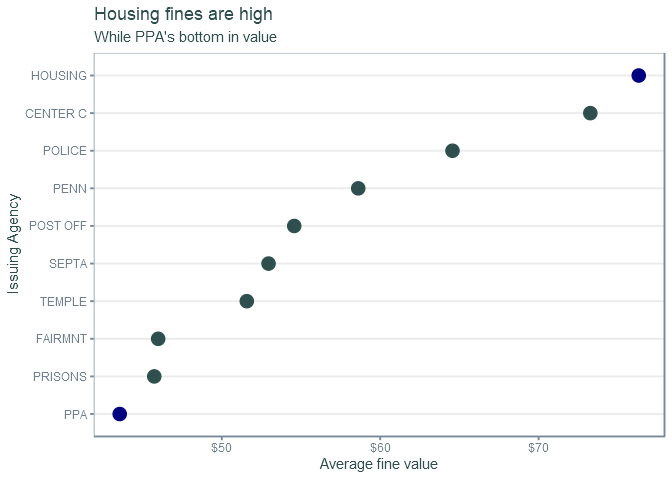
    title = 'Housing fines are high',
    subtitle = 'While PPA\'s bottom in value',
    x = 'Issuing Agency',
    y = 'Average fine value'
  ) +
  coord_flip() +
  scale_y_continuous(labels = scales::dollar_format()) +
  scale_color_manual(values = c('darkslategrey', 'navyblue'), guide = FALSE) +
  theme_bw() + 
  theme(panel.grid.major.x = element_blank(),
        panel.grid.minor = element_blank(),
        strip.background = element_blank(),
        strip.placement = 'outside',
        panel.border = element_rect(color = 'lightslategrey'),
        title = element_text(colour = "darkslategrey"),
        strip.text = element_text(color = 'slategrey'),
        axis.ticks = element_line(color = 'lightslategrey'),
        axis.text = element_text(color = 'slategrey'))

means

total_log <- tickets %>% 
  filter(!is.na(issuing_agency)) %>%
  group_by(issuing_agency) %>% 
  summarise(sum_fine = sum(fine)) %>%
  mutate(housing_ppa = ifelse(issuing_agency %in% c('HOUSING', 'PPA'),
                              'Y', 'N')) %>% 
  ggplot(aes(reorder(issuing_agency, sum_fine), sum_fine,
             color = housing_ppa)) +
  geom_point(size = 4) +
  labs(
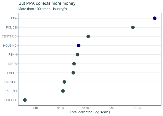
    title = 'But PPA collects more money',
    subtitle = 'More than 100 times Housing\'s',
    x = NULL,
    y = 'Total collected (log scale)'
  ) + 
  coord_flip() +
  scale_y_log10(labels = scales::label_number_si(prefix = '$')) +
  scale_color_manual(values = c('darkslategrey', 'navyblue'), guide = FALSE) +
  theme_bw() + 
  theme(panel.grid.major.x = element_blank(),
        panel.grid.minor = element_blank(),
        strip.background = element_blank(),
        strip.placement = 'outside',
        panel.border = element_rect(color = 'slategrey'),
        title = element_text(colour = "darkslategrey"),
        strip.text = element_text(color = 'slategrey'),
        axis.ticks = element_line(color = 'lightslategrey'),
        axis.text = element_text(color = 'slategrey'))

total_log

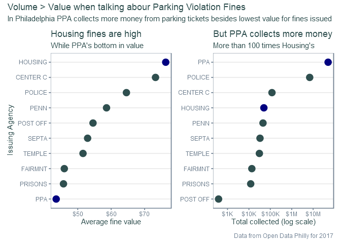
Using patchwork to get the plots together.

final_plot <- means + total_log +
  plot_annotation(
    title = 'Volume > Value when talking abour Parking Violation Fines',
    subtitle = 'In Philadelphia PPA collects more money from parking tickets besides lowest value for fines issued',
    caption = 'Data from Open Data Philly for 2017',
    theme = theme(
      plot.title = element_text(color = 'darkslategrey'),
      plot.subtitle = element_text(color = 'darkslategrey'),
      plot.caption = element_text(color = 'lightslategrey')
      )
    )

final_plot