Tidy Tuesday 05/11/2019 Modes Less Traveled - Bicycling and Walking to Work in the United States: 2008-2012

Data description

From From TidyTuesdays github:

This week’s data is from the ACS Survey. The article and underlying data can be found at the Census Website. The PDF report is also available for download if you’d like to try reading in some of the embedded tables.

Please note that the raw excel files are uploaded (6 total), along with the cleaned/tidy data (commute.csv). There is also a cleaned up version of Table 3 from the article, which incorporates summary data around age, gender, race, children, income, and education for modes of travel (bike, walk, other). If you work with the ACS table 3 I’d suggest dplyr::slice() to grab the specific sub-tables from within it!

Packages and reading data

library(tidyverse)

commute_mode <- read_csv("https://raw.githubusercontent.com/rfordatascience/tidytuesday/master/data/2019/2019-11-05/commute.csv")

First look

commute_mode %>% glimpse()

## Observations: 3,496
## Variables: 9
## $ city         <chr> "Aberdeen city", "Acworth city", "Addison village",…
## $ state        <chr> "South Dakota", "Georgia", "Illinois", "California"…
## $ city_size    <chr> "Small", "Small", "Small", "Small", "Small", "Small…
## $ mode         <chr> "Bike", "Bike", "Bike", "Bike", "Bike", "Bike", "Bi…
## $ n            <dbl> 110, 0, 43, 0, 121, 0, 84, 23, 0, 576, 35, 77, 419,…
## $ percent      <dbl> 0.8, 0.0, 0.2, 0.0, 1.5, 0.0, 0.8, 0.2, 0.0, 1.5, 0…
## $ moe          <dbl> 0.5, 0.4, 0.3, 0.5, 1.0, 0.2, 1.1, 0.3, 0.2, 0.4, 0…
## $ state_abb    <chr> "SD", "GA", "IL", "CA", "MI", "MA", "CA", "SC", "AL…
## $ state_region <chr> "North Central", "South", "North Central", "West", …

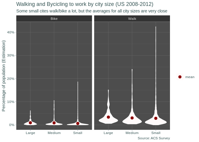
I’ll look the percents, state_regions and city_size.

commute_mode %>% 
  filter(!is.na(state_region)) %>% 
  ggplot(aes(city_size, percent)) +
  geom_violin(color = "white", fill = "snow") +
  stat_summary(fun.y=mean, geom="point", size = 3, aes(group = 1, color = "mean")) +
  labs(
    title = "Walking and Bycicling to work by city size (US 2008-2012)",
    subtitle = "Some small cites walk/bike a lot, but the averages for all city sizes are very close",
    color = NULL,
    x = "City Size",
    y = "Percentage of population (Estimation)",
    caption = "Source: ACS Survey"
  ) +
  scale_y_continuous(labels = scales::percent_format(scale = 1)) +
  scale_color_manual(values = "darkred")  +
  facet_wrap(~mode) +
  theme_dark() +
  theme(
    title = element_text(colour = "darkslategrey"),
    legend.title = element_text(hjust = .5),
    legend.text = element_text(colour = "darkslategrey"),
    axis.ticks = element_line(color = 'lightslategrey'),
    axis.text = element_text(color = 'darkslategrey'),
    axis.line = element_blank(),
    axis.title.x = element_blank(), 
    panel.background = element_rect(fill = "grey30"),
    strip.background = element_rect(fill = "grey20"),
    legend.key = element_rect(fill = "snow")
  )