Tidy Tuesday 06/08/2019 Painting by Numbers
Data description
From TidyTuesdays github:
Each of the columns after episode/title correspond to the binary presence (0 or 1) of that element in the painting.
Import data and packages
library(tidyverse) #data manipulation and ggplot
library(visNetwork) #interactive network
library(igraph) #still newtork
library(tidygraph) #still newtork
library(ggraph) #still newtork
library(Cairo) #render the still newtork

#bob_ross <- readr::read_csv("https://raw.githubusercontent.com/rfordatascience/tidytuesday/master/data/2019/2019-08-06/bob-ross.csv")
#write_csv(bob_ross, "boss_ross.csv")
bob_ross <- readr::read_csv("boss_ross.csv")
Data
Using the recommended steps to break apart the seasons and episodes. Also removing the frame elements.
bob_ross <- bob_ross %>%
  janitor::clean_names() %>%
  separate(episode, into = c("season", "episode"), sep = "E") %>%
  mutate(season = str_extract(season, "[:digit:]+")) %>%
  mutate_at(vars(season, episode), as.integer) %>%
  select(-c(contains("frame"), title))

dim(bob_ross)
## [1] 403 53
Very wide dataframe. Let’s change it to a long, tidy format.
bob_ross <- bob_ross %>%
  gather("element", "presence", -c(season, episode))
This get us a lot of lines with zeroes, let’s dispose of them.
bob_ross <- bob_ross %>%
  filter(presence >0)
EDA
Now a little peek into the data.
bob_ross %>%
  count(element) %>%
  top_n(10, n) %>%
  ggplot(aes(x = reorder(factor(element), n),
             y = n)) +
    geom_col() +
    labs(x = "element", y ="count") +
  coord_flip()
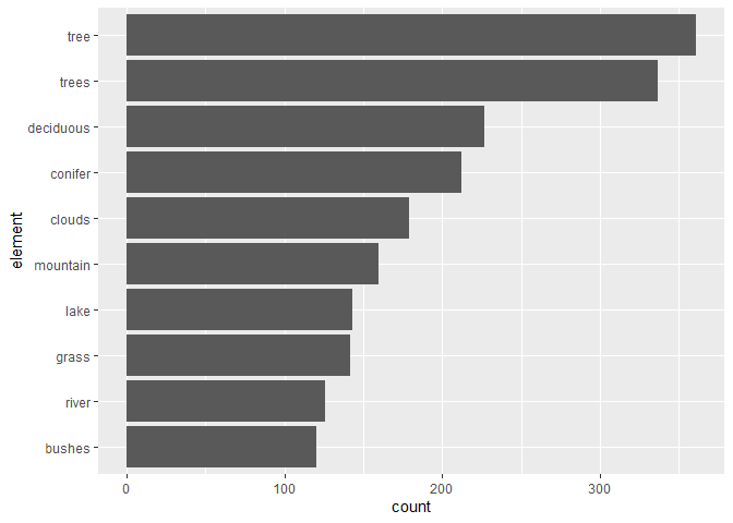
So tree, and trees, are the most common elements. The top 10 elements in general are related with nature, landscapes and backgrounds.
Let’s take a closer look to tree and trees.
bob_ross %>%
  group_by(season, episode) %>%
  summarise(
    only_tree = ifelse(any(element == "tree") & !(any(element == "trees")), 1, 0),
    only_trees = ifelse(!any(element == "tree") & (any(element == "trees")), 1, 0),
    both_tree_trees = ifelse(any(element == "tree") & (any(element == "trees")), 1, 0)
  ) %>%
  ungroup() %>%
  select(-c(season, episode)) %>%
  summarise_all(sum)
Trees is not very informative, since it only says if more than one tree is in the picture and not a really new element. I’ll take away this element and refer to tree as “at least one tree”. And let’s do the same for mountains.
bob_ross <- bob_ross %>%
  filter(element != "trees", element != "mountains")
For this data I chose to represent the most common association of elements, so I’ll use a network graph.
Network graph
Preparing the nodes
First we create a data frame of nodes, with individual ids for each element name (label).
nodes <- bob_ross %>%
  group_by(season, episode) %>%
  mutate(count_el = sum(presence)) %>%
  dplyr::filter(count_el > 1) %>%
  ungroup() %>%
  select(label = element) %>%
  distinct() %>%
  rowid_to_column("id")
So we have 48 unique nodes for our network graph, which is all elements with the exception of lakes, which isn’t present in any painting, trees, mountains and frame elements.
Now preparing the edges. Probably there’s a better way to do this but this large set of steps is what I could come up with. It involves:
- Creating a table with the element counts;
- Join it with itself to create the connections;
- Eliminate the elements’ connections to themselves created by the join.
- Eliminate the mirrored connections. Since join repeats rows that are only a partial match, all combinations are considered and we end up with every connection twice.
- Label the connections with the correct ids.
#Creates a variable of element counts
edges_i <- bob_ross %>%
  group_by(season, episode) %>%
  mutate(count_el = sum(presence)) %>%
  dplyr::filter(count_el > 1) %>% #just to make sure there isn't any element without a connection
  ungroup() %>%
  select(-c(presence,count_el))

#Creates a table of top 100 connections and their sizes
edges <- edges_i %>%
  inner_join(edges_i, by = c("season", "episode")) %>%
  dplyr::filter(element.x != element.y) %>%
  group_by(grp = paste(pmax(element.x, element.y), pmin(element.x, element.y), sep = "_"), season, episode) %>%
  slice(1) %>%
  ungroup() %>%
  select(-c(grp, season, episode)) %>%
  group_by(element.x, element.y) %>%
  summarise(value = n()) %>%
  ungroup() %>%
  top_n(100, value)

#Label the connections correctly
edges <- edges %>%
  left_join(nodes, by = c("element.x" = "label")) %>%
  rename(from = id) %>%
  left_join(nodes, by = c("element.y" = "label")) %>%
  rename(to = id) %>%
  select(from, to, value)
Then we’ll look into the nodes again to only select the nodes that appear in the top 100 connections, so we don’t have any isolated node in the network.
#Get only the nodes that are in the top 100 connections
nodes_chosen <- nodes %>%
  dplyr::filter(id %in% c(edges$from, edges$to))

#Variable for size of the nodes
nodes_chosen$size <- bob_ross %>%
  dplyr::filter(presence == 1) %>%
  count(element) %>%
  inner_join(nodes_chosen, by = c("element" = "label")) %>%
  .$n/10
Create the interactive network
With visNetwork package it’s easy to create a network element. But I had to try it some times to choose a good seed and solver algorithm and parameters. I did also some modifications of some css elements to make the plot look better, they don’t change the plot made in the .Rmd or in R but they are displayed in the html document.
I haven’t found a way to make annotations, so I tried to give the minimum relevant information in the title and subtitle. And fade them a little so they don’t take attention away from the data.
#create visualization
#Html content. Not run in the md.
visNetwork(nodes_chosen, edges,
           main = list( text = "What elements does Bob Ross paint together?",
                        style = 'font-family:Georgia, Times New Roman, Times, serif;
                        font-weight:bold;font-size:20px;text-align:left;color:slategray;'
                        ),
           submain = list(text = 'Close circles have similar pairings, large circles are
                          common elements, thick lines are common pairings' ,
                          style ='font-family:Georgia, Times New Roman, Times, serif;
                          font-size:13px;text-align:left;color:slategray'
                          )
           )%>%
  visNodes(color = list(background = "steelblue",
                        border = "lightblue",
                        highlight = "orange"),
           font = list(size = 16)
           ) %>%
  visEdges(color = list(color = "lightblue", highlight = "steelblue")
           ) %>%
  visPhysics(solver = "forceAtlas2Based",
             forceAtlas2Based = list(gravitationalConstant = -22)
             )%>%
  visLayout(randomSeed = 100) %>%
  visInteraction(navigationButtons = TRUE)
Creating a still network
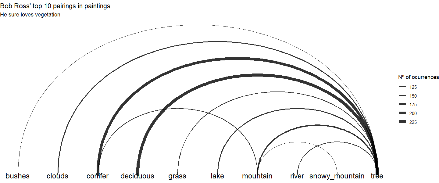
I also created a still network using ggraph package, but the image didn’t render nicely using windows, just improved a little using the Cairo package.
First I do some of the steps as above to create a selection of nodes and edges of the top 10 connections.
edges <- edges %>%
  top_n(10, value)


nodes_chosen <- nodes %>%
  dplyr::filter(id %in% c(edges$from, edges$to))

nodes_chosen$size <- bob_ross %>%
  count(element) %>%
  inner_join(nodes_chosen, by = c("element" = "label")) %>%
  .$n/10
Then I create an igraph element to map the nodes and edges.
br_igraph <- graph_from_data_frame(d = edges[,1:3], vertices = nodes_chosen[,1:2], directed = TRUE)

br_tidy <- as_tbl_graph(br_igraph)
Then I create the gggraph network.
windowsFonts("Arial Narrow" = windowsFont("Arial")) #Making it recognize windows fonts

ggraph(br_tidy, layout = "linear") +
  geom_edge_arc(aes(width = value), alpha = 0.8) +
  scale_edge_width(range = c(0.2, 3)) +
  geom_node_text(aes(label = label), size = 5) +
  labs(title = "Bob Ross' top 10 pairings in paintings",
       subtitle = "He sure loves vegetation",
    edge_width = "Nº of ocurrences") +
  theme_void()