Tidy Tuesday 22/10/2019 Horror Movies Metadata

Data description

From From TidyTuesdays github:

This week’s data is from the IMDB by way of Kaggle.

H/t to Georgios Karamanis for sharing the data this week.

Thrillist did a 75 Best Horror Movies of all Time article. There’s also a Stephen Follows article about horror movies exploring data around profit, popularity and ratings.

Last year for Halloween we focused on Horror Movie Profit - feel free to take a peek at that data as well on our GitHub.

Import data and packages

library(tidyverse) #data collection, manipulation and plots
library(tidytext) #text manipulation
library(scales) #number format transforming
library(here) #make sure the figures are in the right place
library(RCurl) #because curl is giving me a headache

horror_movies <- readr::read_csv(RCurl::getURL(
  "https://raw.githubusercontent.com/rfordatascience/tidytuesday/master/data/2019/2019-10-22/horror_movies.csv"
  ))

Data

glimpse(horror_movies)

## Observations: 3,328
## Variables: 12
## $ title             <chr> "Gut (2012)", "The Haunting of Mia Moss (2017)…
## $ genres            <chr> "Drama| Horror| Thriller", "Horror", "Horror",…
## $ release_date      <chr> "26-Oct-12", "13-Jan-17", "21-Oct-17", "23-Apr…
## $ release_country   <chr> "USA", "USA", "Canada", "USA", "USA", "UK", "U…
## $ movie_rating      <chr> NA, NA, NA, "NOT RATED", NA, NA, "NOT RATED", …
## $ review_rating     <dbl> 3.9, NA, NA, 3.7, 5.8, NA, 5.1, 6.5, 4.6, 5.4,…
## $ movie_run_time    <chr> "91 min", NA, NA, "82 min", "80 min", "93 min"…
## $ plot              <chr> "Directed by Elias. With Jason Vail, Nicholas …
## $ cast              <chr> "Jason Vail|Nicholas Wilder|Sarah Schoofs|Kirs…
## $ language          <chr> "English", "English", "English", "English", "I…
## $ filming_locations <chr> "New York, USA", NA, "Sudbury, Ontario, Canada…
## $ budget            <chr> NA, "$30,000", NA, NA, NA, "$3,400,000", NA, N…

I think I’ll go for some text mining and look for the plots. First some tokenizing.

#creating a ata frame with digrams
horror_token <- horror_movies %>% 
  select(plot, genres) %>%
  unnest_tokens("genre", genres, token = "ngrams", n =2) %>% 
  filter(str_detect(genre, "fi", negate = TRUE),
         str_detect(genre, "horror")) %>% 
  distinct()

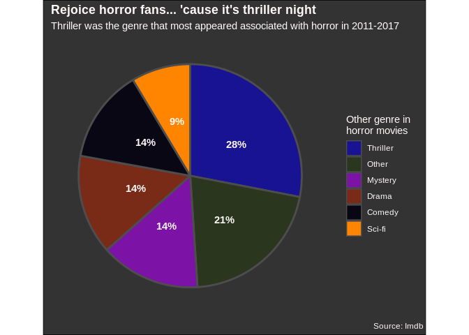
I’ll make a pie chart with the proportion of released movies in all years. But first I have to create the labels.

#vector with the 5 most common digrams
most_common <- horror_token %>% 
  group_by(genre) %>% 
  summarise(n = n()) %>% 
  top_n(5, n) %>% 
  select(genre) %>% 
  as_vector() %>% 
  unname()

#fucntion to capitalize categories. Stolen from R 
 .simpleCap <- function(x) {
    s <- strsplit(x, " ")[[1]]
    paste(toupper(substring(s, 1, 1)), substring(s, 2),
          sep = "", collapse = " ")
}

Then I create a table with the proportion of each of the selected categories.

 horror_token %>% 
  mutate(top = case_when(
    genre == "horror sci" ~ "Sci-fi",
    genre %in% most_common ~  str_remove(genre, "\\s?horror\\s?"),
    TRUE ~ "Other"
  )) %>%
  group_by(top) %>%
  count() %>% 
  ungroup() %>% 
  transmute(n = n/sum(n),
            top = map_chr(top, .simpleCap),
         top = fct_reorder(top, n)) %>% 
  ggplot(aes(x = "", y = n, fill = top)) +
  geom_bar(stat = "identity", width = 1, size = 1, color = "grey30") +
  geom_text(aes(label = percent(n, accuracy = 1)),
            position = position_stack(vjust = .55),
            color = "snow", fontface = "bold") +
  labs(
    title = "Rejoice horror fans... \'cause it\'s thriller night", 
    subtitle = "Thriller was the genre that most appeared associated with horror in 2011-2017",
    fill ="Other genre in \nhorror movies",
    caption = "Source: Imdb"
  ) +
  guides(fill = guide_legend(reverse = TRUE, override.aes = c(size = .5))) +
  scale_fill_manual(values = c("#FF8500", "#090714", "#792B17",
                               "#7C12A6", "#2A361E", "#181393")) +
  coord_polar("y", start = 0) +
  theme_minimal() +
  theme(
    plot.background = element_rect(fill = "grey20"),
    plot.title = element_text(color = "snow", face = "bold"),
    plot.subtitle = element_text(color = "snow"),
    plot.caption = element_text(color = "snow",
                                hjust = 1.41),
    panel.grid = element_blank(),
    legend.background = element_rect(fill = "grey20",
                                     color = "grey20"),
    legend.text = element_text(color = "snow"),
    legend.title = element_text(color = "snow"),
    legend.box.margin = margin(1,3,1,1),
    axis.line = element_blank(),
    axis.text = element_blank(),
    axis.title = element_blank()
  )